How To Find Missing Values Between 2 Columns In Excel
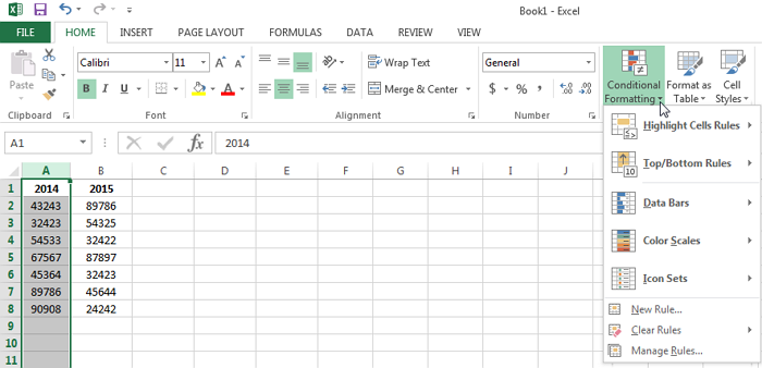
Compare two lists and adding missing values with a handy comparing tool If you have Kutools for Excel installed in Excel you can use the Select Same Different Cells utility to quickly find the missing data between two lists then copy and paste them to the shorter list one. In the Styles group click on the Conditional Formatting option.
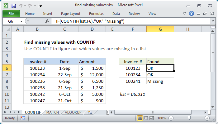
Excel Formula Find Missing Values Exceljet
Hover the cursor on the Highlight Cell Rules option.

How to find missing values between 2 columns in excel. Compare Two Columns to Find Missing Value by Conditional Formatting. SMALL IF COUNTIF List1 ROW INDEX AA F2INDEX AA F3COUNTIF List2 ROW INDEX AA F2INDEX AA F30 ROW INDEX AA F2INDEX AA F3 ROW A1 How to create an array formula Select cell B5 Press with left mouse button on in formula bar. In the Format values where this formula is true field enter the formula.
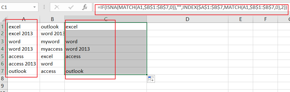
Sometimes you may want to find the duplicate values in a column the Kutools for Excel also can help you quickly handle it. First you can copy the two columns of data and paste them into column A and Column C separately in a new worksheet leave Column B blank to put the following formula. Using the MATCH function with ISNA and IF function to find missing values.
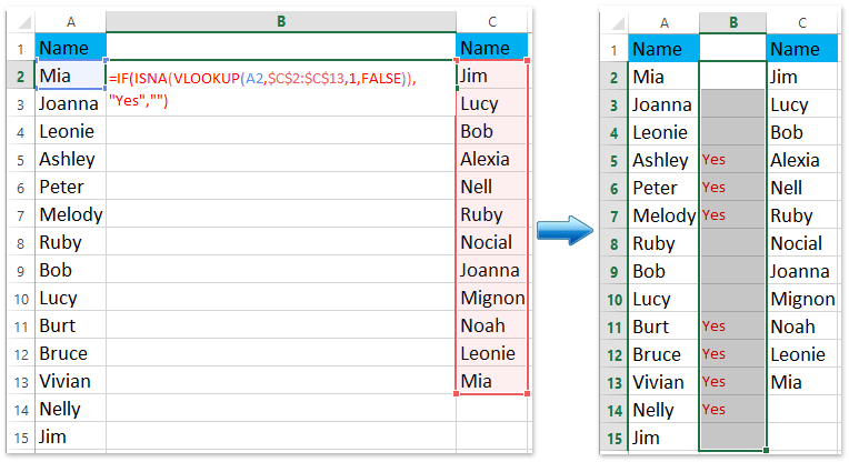
Missing values can also be found with the help of VLOOKUP function. The video offers a short tutorial on how to find missing values between two lists in Excel. In Duplicate Values dialog select Unique in dropdown list.
VLOOKUP returns a NA error if a value. In the example shown the last value in list B is in cell D11. Values that are missing.
Keep default value in values with. This formula is useful when comparing two lists to find out what cell values are missingFor instance inventory comparison. The COUNTIF function lets you compare values if you enter it as an array formula and use multiple values as criteria.
You can use behavior directly inside an IF statement to mark values that have a zero count ie. INDEXB3B18 SMALLIFISERRORMATCHB3B18 D3D6 0 ROWB3B18-MINROWB3B181 ROWSA1A1. FilterA2A13isnamatchA2A13B2B110 into cell C2 and then press Enter key all values in List 1 but not in List 2 are extracted as following screenshot shown.
IFCOUNTIF list F6 OKMissing where list is a named range that corresponds to the range B6B11. In the example shown the formula in G6 is. IF ISNA MATCH valuerange0MISSINGOK The results obtained by this function are the same as shown below.
Click Home in ribbon click Conditional Formatting in Styles group. Summary To compare two lists and extract common values you can use a formula based on the FILTER and COUNTIF functions. COUNTIF range criteria COUNTIF D3D12 B3B12 becomes.
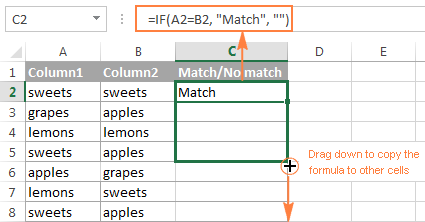
A2B2 Click on the Format button Click on the Fill tab and select the color in which you want to highlight the rows with the same value in both columns. Compare and extract the missing values from two columns with formula If you want to compare and extract the missing values from two columns here is another formula to help you. In the example shown the formula in F5 is.
In Conditional Formatting dropdown list select Highlight Cells Rules-Duplicate Values. The generic formula for finding the missing values using the MATCH function is written below. Summary To compare two lists and pull missing values from one list to the other you can use an array formula based on INDEX and MATCH.
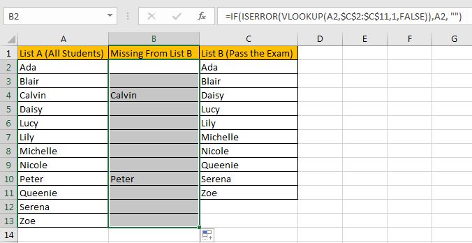
To check if the values are in another column in Excel you can apply the following formula to deal with this job. Sub CompareLists ApplicationScreenUpdating False Dim LastRow As Long LastRow CellsFind SearchOrderxlByRows SearchDirectionxlPreviousRow Dim Rng As Range RngList As Object Set RngList CreateObjectScriptingDictionary With SheetsFeuil1 For Each Rng In RangeA2 RangeA RowsCountEndxlUp If Not RngListExistsRngValue Then RngListAdd RngValue. Select the first blank cell besides Fruit List 2 type Missing in Fruit List 1 as column header next enter the formula IF ISERROR VLOOKUP A2Fruit List 1A2A221FALSEA2 into the second blank cell and drag the Fill Handle to the range as you need.
Select the entire data set. Select List A and List B. Click the Home tab.
Select the column you want to find duplicate values click Kutools Select Select Duplicate Unique Cells. The formula in D12 copied down is. Step 1 - Compare cell range 1 with cell range 2.

How To Compare 2 Columns With Excel So Easy With Only 2 Functions

How To Find Missing Numbers In A Sequence Number Sequence Excel Missing Numbers
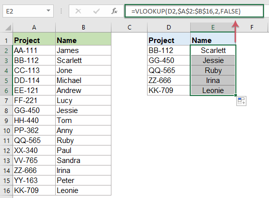
How To Compare Two Columns And Return Values From The Third Column In Excel
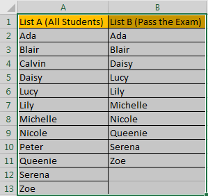
How To Compare Two Columns To Find Missing Value Unique Value In Excel Free Excel Tutorial
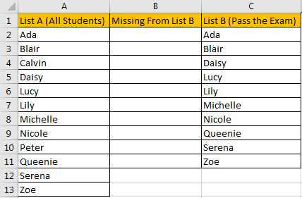
How To Compare Two Columns To Find Missing Value Unique Value In Excel Free Excel Tutorial

How To Compare Two Columns For Highlighting Missing Values In Excel

How To Compare Two Excel Sheets For Differences
How To Align Duplicate Values Within Two Columns In Excel Free Excel Tutorial
How To Find Unique Duplicate Values Between Two Columns In Excel
How To Compare Two Columns To Find Missing Value Unique Value In Excel Free Excel Tutorial

How To Compare Two Columns For Highlighting Missing Values In Excel
Excel Compare Two Columns For Matches And Differences

How To Compare Two Columns For Highlighting Missing Values In Excel
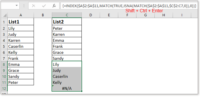
Compare Two Columns And Add Missing Values In Excel
Compare Two Columns And Remove Duplicates In Excel Excel Excel Formula Microsoft Excel

How To Compare 2 Columns With Excel So Easy With Only 2 Functions
How To Compare Two Columns To Find Duplicates In Excel Excel Tutorial For Excel 2013

How To Use Division Formula In Excel Microsoft Excel Excel Tutorials Microsoft Excel Tutorial

How To Compare 2 Columns With Excel So Easy With Only 2 Functions